The validation story

Every solver page on the internet says “validated against NEC”. This page is the longer version: what antennaknobs’ numbers are checked against, what the checks found — including the defects they found on our side — and exactly which claims stop where. The short version of the claim:

• Parity on plain geometries, grounds and patterns: three independently derived, independently coded formulations agree — momwire’s B-splines, the NEC-2 lineage, and NEC-5’s mixed-potential formulation (0.01 dB RMS class on far-field patterns, a few ohms of genuine formulation spread on impedance).
• Superiority where the reference is wrong: on stepped-diameter elements the NEC-2 lineage carries a known defect (the reason EZNEC ships the Leeson correction). There, momwire and NEC-5 agree against the two NEC-2 implementations — the correction table is built into the physics.
• Honest limits, stated up front: what antennaknobs does not model, it refuses by name — never a silently simplified answer. The limits table is part of the validation story, not a footnote.

The method

The cross-checking machinery is described on the solver & accuracy and NEC-5 engine pages; the short form:

• Three formulations that share almost nothing. momwire (sinusoidal and B-spline Galerkin bases), NEC-2 (nec2c and nec2++, thin-wire collocation), and NEC-5 (LLNL’s modern mixed-potential rewrite). When they agree, the agreement means something; when they split, the split is a finding to run down — several of the findings below started life as “our bug” and ended as a documented property of the reference.
• The census metric is ΔΓ: the distance between reflection coefficients at 50 Ω. Unlike raw ohms it is bounded, comparable across feed impedances from an ohm to ten thousand, and weighted the way a transmitter sees the antenna.
• Census-grade NEC-5 numbers are Richardson (N, 2N) pairs. NEC-5’s knot-source discretization converges first-order in segment length — LLNL’s own Validation Manual describes the behaviour (Burke & Poggio, NEC 5.0, LLNL-CODE-746721) — so the census extrapolates a native and a doubled-mesh solve rather than quoting either raw read. The NEC-5 page tells the full story of how that recipe was pinned.

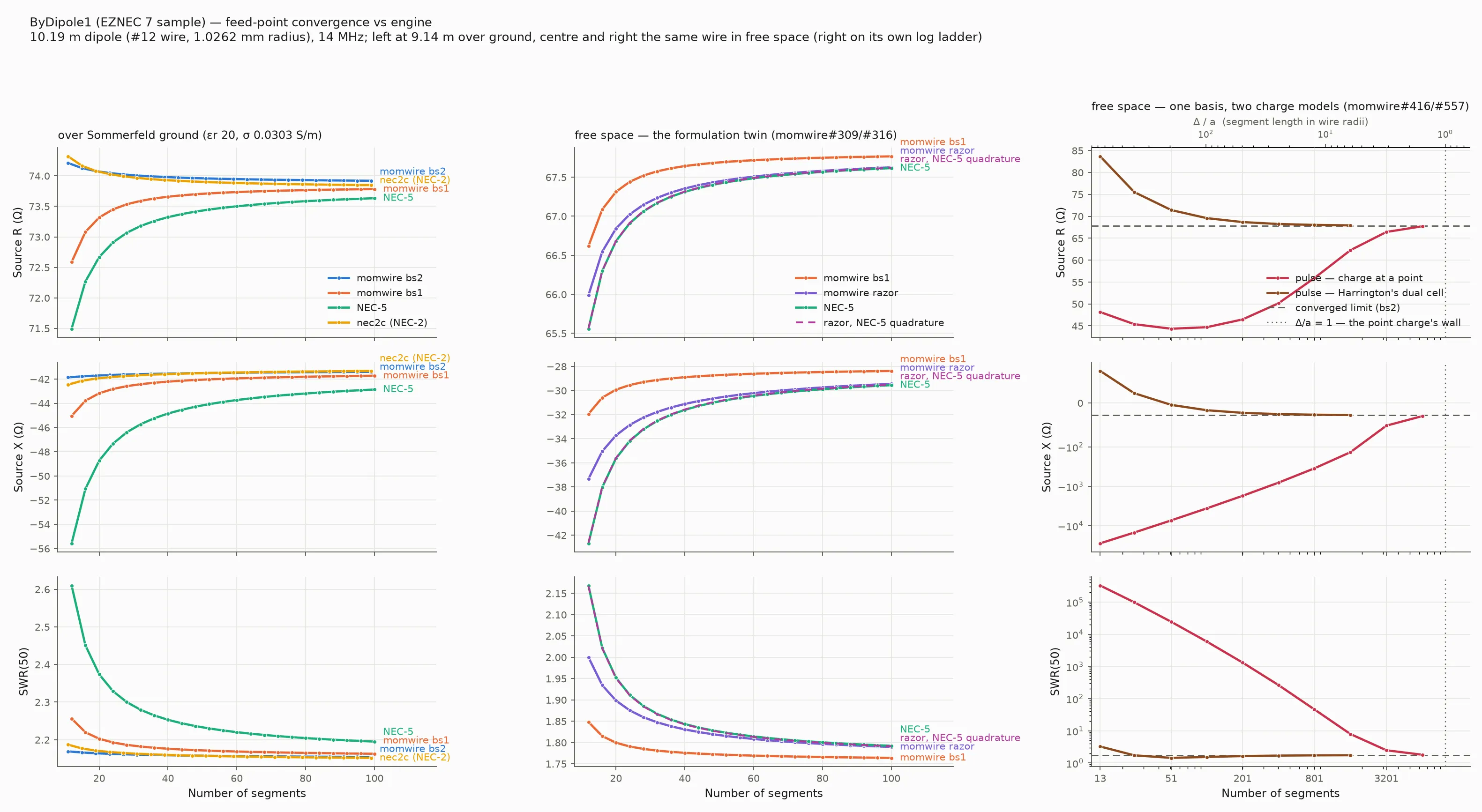
Case: ByDipole1 — the EZNEC sample everyone can re-run

ByDipole1 ships with EZNEC 7: a 10.19 m dipole at 9.144 m height, #12 wire (1.0262 mm radius), 14 MHz, over real Sommerfeld ground (εr 20, σ 0.0303 S/m). It is a community-recognizable case — NEC-2 vs NEC-5 convergence plots for it were independently published by AC6LA — and it sits squarely in NEC-2’s good regime (single radius, no junctions), which makes it a convergence-rate exhibit: every engine here converges to the same answer, and the question is how many segments each needs to get there.

engine	coarsest read — Z in Ω (SWR₅₀) @ N	finest read @ N
momwire bs2	74.21 -41.85j (2.17) @ 11	73.92 -41.40j (2.15) @ 99
momwire bs1	72.59 -45.04j (2.26) @ 12	73.78 -41.72j (2.16) @ 100
nec2c (NEC-2)	74.32 -42.45j (2.19) @ 11	73.85 -41.32j (2.15) @ 99
NEC-5 raw	71.49 -55.57j (2.61) @ 12	73.63 -42.86j (2.20) @ 100

NEC-5 (N, 2N) pair extrapolations: (44,88) → 73.84 -41.54j / (48,96) → 73.84 -41.55j — both pairs land on the common limit within 0.05 Ω of each other.

What the plot shows:

• Three formulations converge to a common limit within ~0.2 Ω on a real-ground sample they did not choose.
• bs2 at eleven segments reads 74.21 -41.85j — within 0.4 Ω and 0.014 SWR of the limit. That is the flat line in the figure, and it is what “census-grade at coarse mesh” means in practice.
• Raw NEC-5 at twelve segments reads 71.49 -55.57j (SWR 2.61) and needs N≈100 to close within 1.5 Ω (73.63 -42.86j); the (N, 2N) pair recipe recovers the limit from either half of the ladder. This is NEC-5’s documented first-order knot-source march, not an error — but it is why quoting a single raw NEC-5 read at low N misleads.
• Independent cross-check of our NEC-5 lane: the same runs reproduce AC6LA’s published EZNEC-Pro NEC-5 curves to plot-reading precision — our runner and a second, unrelated NEC-5 host produce the same numbers from the same physics.

The centre column is the same wire in free space, and it explains WHY NEC-5 marches. NEC-5’s public manual states its formulation — a triangular (tent) current expansion tested by Rao-Wilton-Glisson path integrals between element centroids (“razor-blade” testing) — and momwire now implements that exact scheme as RazorSolver, the formulation twin (momwire#309). On identical meshes the twin shares NEC-5’s first-order march — X-pair steps X(2N)−X(N) of +4.49 / +2.18 / +1.17 Ω against NEC-5’s +8.50 / +3.16 / +1.41 Ω at N=12/24/48, the same halving-per-doubling signature (NEC-5 carries extra coarse-mesh excess on the first pair) — and the two curves land together on a common limit, while bs1, the same tent basis under Galerkin testing, converges visibly faster on its own trajectory. The march is the testing rule, reproduced from the manual’s description alone, with no NEC-5 code involved.

The dashed overlay closes the loop: NEC-5’s remaining coarse-mesh excess over the twin was identified (momwire#316) as its quadrature — the ∫A·dl testing integral evaluated by a two-point trapezoid at the element centroids, the literal reading of “path integrals between centroids”. With that one rule adopted (nec5_quadrature=True), the razor lane lands on NEC-5’s curve at every rung, to a constant −0.004−0.037j Ω — an N-independent kernel nuance and the entire remaining difference between the two codes on this wire. (The twin panel is free-space by choice, not necessity: RazorSolver serves the PEC and Sommerfeld grounds, and razor-2p is the app’s above-ground lane over both. NEC-5’s Michalski ground has its own small limit offset that would blur the formulation comparison, so the twin is compared where the formulation is the only difference.)

What the charge model is worth: one basis, two ways to place it

The right-hand column holds the oldest thin-wire scheme there is — Harrington’s piecewise-constant current, point-matched, 1967 — twice. Both lanes use the same basis, the same testing, the same kernel and the same feed. They differ in one thing: where the charge lives.

A pulse current is discontinuous, so its charge is exactly two spikes at the segment ends. You can take that literally and put a point charge there, which is what momwire’s PulseSolver does. Or you can do what Harrington’s paper actually specifies — spread each one over a half-shifted cell straddling the node, his equations (95)/(96)/(100) — which is HarringtonSolver. Everything else about the two rows is the same code.

Segments	Δ/a	charge at a point	error	Harrington’s dual cell	error
13	763.8	48.15 -27987.58j	27,959.7	83.67 +73.28j	102.39
25	397.2	45.38 -14926.38j	14,898.5	75.53 +22.46j	50.93
51	194.7	44.34 -7331.53j	7,303.7	71.42 -4.18j	23.97
101	98.31	44.69 -3632.16j	3,604.3	69.58 -16.38j	11.64
201	49.4	46.47 -1748.57j	1,720.8	68.68 -22.36j	5.60
401	24.76	50.14 -809.91j	782.2	68.24 -25.25j	2.67
801	12.4	55.91 -351.02j	323.3	68.03 -26.63j	1.28
1601	6.202	62.26 -136.75j	109.0	67.93 -27.26j	0.63
3201	3.102	66.42 -51.58j	23.7	—	—
6401	1.551	67.73 -29.72j	1.8	—	—
limit (bs2, N=401)	—	67.86 -27.89j	—	—	—

That is a factor of 310× between two solvers that differ by one modelling decision, and it is the sharpest statement this page can make about why formulations are worth arguing over. Neither lane is wrong about the physics; both walk to the same limit. One of them just needs 310 times the accuracy budget to get there.

Why the point charge costs so much. Its error is governed by Δ/a — segment length in wire radii — not Δ/λ. A point charge’s potential at its own location is finite only because the thin-wire kernel floors the distance at the conductor radius, so the mesh has to approach the radius before that error retires. ByDipole1’s wire is 1.0262 mm in radius — #12 AWG — which puts Δ/a = 1 at about 9,929 segments — the dotted vertical — and refining past it does not merely stop helping, it reverses. The usable window is the sliver between that wall and a mesh nobody would pay for.

Give the charge a cell of its own length and the wire radius stops setting the scale. The dual-cell lane converges O(1/N) like any classical scheme, reaching 0.63 Ω at 1,601 segments, with no wall anywhere on the axis.

What this column is not. It is not a claim that the 1967 scheme is obsolete — momwire ships it as HarringtonSolver, and it is a perfectly reasonable base case. (PulseSolver, the point-charge lane beside it, is momwire’s own literal reading of the same basis, not Harrington’s scheme; neither is in the app’s --basis roster.) It is a control: the two panels to its left vary the basis and the testing, and this one varies neither. Whatever separates these two curves cannot be blamed on either, which is what makes the number mean something. Harrington’s own advice, on page 145 of the same paper, is to move on anyway: “faster convergence can be obtained by going from a step approximation to a piecewise-linear approximation to the current” — the tent basis, which is the bs1 lane in the middle column.

Provenance: geometry translated from the EZNEC 7 distribution, with EZNEC’s current-source feed idiom replaced by a direct center voltage feed (driving-point impedance is source-type independent; the equivalence is pinned in the test suite). The NEC-2 curve is nec2c — the same lineage as EZNEC’s NEC-2D, independently implemented. The razor lane is momwire’s RazorSolver on the momwire#311 branch. The two pulse lanes are momwire’s PulseSolver and HarringtonSolver (momwire#557); the point-charge lane’s 6401-segment rung is a 6401×6401 dense solve, about 40 s and 5 GB, and the dual-cell lane stops at 1601 because its charge cells make the moment block twice as wide in each direction, and by then it is inside an ohm of the limit — still halving per rung, but far below anything the figure’s axes can show.

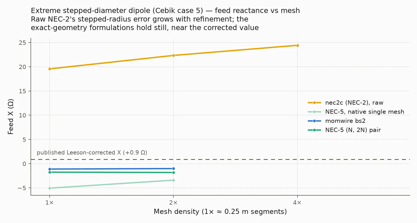
Case: the Leeson demo — stepped-diameter elements

Practical Yagi elements taper: fat tubing at the boom, thinner sections toward the tips. NEC-2 carries a documented defect at wire-radius steps — serious enough that EZNEC ships a correction (David Leeson’s uniform-diameter substitute elements) and applies it whenever a stepped element qualifies. L.B. Cebik (W4RNL) published the canonical demonstration: five 14 MHz free-space dipoles with progressively harder tapers, giving uncorrected and Leeson-corrected NEC-2 values for each (“Tapering to Perfection”, Antenna Modeling #10). Here are his cases through our engines — the exact stepped geometry, no correction applied anywhere:

element (14 MHz, free space)	published NEC-2 raw	our nec2c, 1×→4× mesh	momwire bs2	NEC-5 pair	published corrected
uniform 1.0″	—	72.03 +0.63j → 72.28 +1.26j	72.01 +0.24j	72.03 -0.01j	71.80 -0.60j
one step, far out	73.00 +4.40j	73.55 +7.22j → 74.44 +10.92j	72.01 -2.09j	72.01 -2.33j	72.00 +0.40j
one step, near center	72.40 +5.20j	72.40 +7.66j → 72.38 +10.52j	73.50 -0.40j	73.51 -0.64j	71.80 -0.50j
two steps, modest taper	72.50 +10.60j	72.42 +12.71j → 72.46 +17.34j	73.87 -1.43j	73.87 -1.73j	71.90 +0.10j
two steps, extreme taper	67.60 +17.10j	66.56 +19.56j → 65.29 +24.42j	76.55 -1.02j	76.53 -1.83j	72.10 +0.90j

Reading the table:

• The control row behaves: on the uniform element every engine and the published value agree within a few tenths of an ohm.
• Our raw nec2c reproduces the published defect, and the mesh march shows something the single published number cannot: the error grows as you refine the mesh. On the extreme taper the reactance error runs +19.6 Ω at 1× density to +24.4 Ω at 4× — you cannot mesh your way out of a formulation defect. (Our reads differ from Cebik’s published raw values by a few ohms of X because the raw error is segmentation-dependent and his segment counts were not published; the signature and direction match throughout.)
• The two exact-geometry formulations agree with each other — bs2 and the NEC-5 pair land within 0.81 Ω on every case — and sit where the correction points: reactance within 2.5 Ω of the corrected value on every taper. The correction table is built into the physics.
• On the extreme taper the corrected resistance sits ~4 Ω from the exact-geometry consensus — a reminder that the Leeson correction is itself an approximation (a uniform substitute element), and two independent formulations solving the true geometry is the stronger statement of the two.

This is the same defect the wild-corpus census found at scale — see the next section: 44 of the 46 formulation-line movers are stepped-radius decks.

The wild-corpus census

The strongest evidence is not a curated demo but a corpus nobody tuned: 3,146 wire decks collected from public archives (ARRL, Cebik, tutorial collections, community files), each solved by multiple engines and scored pairwise :

• NEC-5 solved 2,314 decks as (N, 2N) pairs with zero unclassified errors; 488 decks refused by design (dialect features like TL/NT the engine names rather than approximates).
• Clean-cohort median ΔΓ against nec2c: bs2 0.0080 (n=1686), NEC-5 pairs 0.0215 (n=1369).
• At the ΔΓ > 0.2 outlier bar, the clean three-way cohort (1,368 decks) splits into: 2 decks where momwire is the outlier (filed and tracked as momwire defects — that is the entire momwire-suspect pile after five phases of hunting), 10 where NEC-5’s pair is under-resolved (pre-asymptotic decks, a practical-limits note), and 61 where bs2 and NEC-5 agree with each other against nec2c.

Those 61 mutually-agreeing decks got a fourth vote — nec2++ (PyNEC), which shares geometry translation with the momwire lane but formulation with nec2c, so it discriminates translation bugs from formulation findings. Of the 47 decks it could score: 46 split along formulation lines ({bs2 + NEC-5} vs {nec2c + nec2++} on identical geometry), 1 translation-suspect. And 44 of the 46 have stepped or multi-radius elements — the documented NEC-2 stepped-diameter defect, corrected in NEC-4/NEC-5 and by EZNEC’s Leeson option. On those decks the census now flags the reference as suspect and scores bs2 against NEC-5 instead (mutual ΔΓ 0.004-class where nec2c sits 0.2–0.3 away).

The census also cut both ways — the machinery found and fixed defects on our side (a wire-connection snap in deck import, two momwire solver issues filed from census evidence) and the historical scoring was rewritten against us where the reference was wrong. An audit trail that only ever vindicates its author is not an audit trail.

Convergence at fixed mesh

From the committed convergence census (13 designs across the catalog’s families — loops, yagis, folded elements, multi-junction fans, loaded short antennas), each engine’s self-movement between its coarsest and finest ladder rung (ΔΓ between the N=21 and N=161 reads; smaller = already converged at coarse mesh):

design	NEC-5 raw	momwire bs2	momwire sin
specialty.hentenna	0.0467	0.0030	0.0172
loops.quad	0.0061	0.0017	0.0018
loops.delta_loop	0.0045	0.0006	0.0075
loops.bisquare	0.0015	0.0014	0.0020
multiband.fandipole	0.0193	0.0609	0.1671
dipoles.folded_invvee	0.0022	0.0015	0.0041
beams.yagi	0.0489	0.0096	0.0083
beams.moxon	0.0624	0.0083	0.0144
dipoles.invvee	0.0245	0.0048	0.0054
dipoles.ocf_dipole	0.0121	0.0003	0.0040
verticals.bruce	0.0006	0.0020	0.0017
verticals.jpole	0.0263	0.0034	0.0307
dipoles.short_dipole_loaded	0.2620	0.4037	0.5606

bs2’s coarse read is already census-grade (self-ΔΓ ≤ 0.01) on 11 of 13 designs. The exceptions are honest: the fandipole’s near-open parallel resonance and the loaded short dipole move under every engine — those are genuinely mesh-hard designs, and the raw NEC-5 column shows the first-order march the (N, 2N) pair recipe exists to remove.

Honest limits

What antennaknobs will not claim, in one table. Refusal-over-wrong is a design decision: where a number would be misleading, you get a named refusal or a flag, not a number.

limit	treatment
Surface patches (SM/SP)	Not modelled. Patch decks refuse at import with the feature named.
Buried wires / below-ground conductors	Served on the momwire bspline lane over the Sommerfeld ground: impedance, currents and charges for wires strictly below the interface (buried radials and screens, buried fed elements, elevated feeds over buried counterpoises), and an above-ground wire joined at the surface to buried wires at a declared junction (the connected radial screen). Refused by name: a wire crossing the interface mid-span; ground-contact wires mixed with buried wires; a wire lying in the interface plane (the surface class — radials lying on the ground — is served instead as the elevated family at an explicit small height, momwire#872; see below); a buried structure whose opposite tips are more than 4 in-medium wavelengths apart (the below/below remainder is tabulated to that range and grows with distance beyond it, so there is no honest clamp); and near fields / patterns of buried decks. A licensed local NEC-5, asked with its documented below-ground card, agrees with momwire on the buried-radial vertical’s connected deck to 2.6 % in resistance at the design’s defaults (77.8+44.5j against 75.8+40.5j Ω) and on the wholly buried dipole to 0.2 % in resistance across depths; on the elevated-detached class, which both serve as the same problem, they agree at the 0.2–2 Ω level converged (the buried-radials study). The one buried spelling NEC-5 has no documented answer for is a conductor stopping on the interface above buried wires (the detached variant), which momwire refuses by name on its own physics. The PyNEC lane is gated off buried decks: nec2++ solves a buried wire as though it were in air and returns a plausible number, so the app withholds it with a sentence rather than serve it. The validation stance below ground is its own paragraph under this table.
Electrically tiny, fat-conductor loops (magloop class)	Kernel-sensitive beyond any single-kernel read — reduced vs extended thin-wire kernels move results both ways by amounts that swamp formulation agreement. Census rows carry a kernel-sensitivity flag rather than a false-precision number.
sin basis on junction fans	A documented instability class on multi-wire junction geometries. bs2 is the default and census basis; sin remains available with the caveat attached.
Stepped-radius decks scored against NEC-2 references	The reference is the suspect (two independent formulations agree against it). Census rows carry the stepped-radius flag and score against NEC-5 mutually instead of pretending the nec2c number is truth.
wire.sterba_bl on the momwire razor lanes	Not served, at any mesh, with or without ground. The deck carries a junction PORT, and a junction basis is already a through-current unknown, so the razor formulation has nowhere to put one — it refuses by name with junction_ports rather than quietly dropping the port. bspline serves the deck normally, and is the lane the census uses for it.

Below the interface, validation stands on two legs. The engine-independent gates are exact identities: the lossless-limit collapse onto the free-space solve, the deep-burial limit onto the infinite-medium solve, and a quasi-static two-electrode cross-estimate — plus, on the buried radial and counterpoise classes, ladder-limit agreement at the half-percent class with the with/without-radials coupling differential matching to about a milliohm. The cross-engine leg is a licensed NEC-5 asked with its documented below-ground card: on the wholly buried fed dipole the two engines agree to 0.2 % in resistance at 0.15, 1 and 2 m depth (146.4+44.4j against 146.6+44.7j Ω at 0.15 m), and on the bonded-base vertical over buried radials to 2.6 % at four radials and 3.9 % at twelve.

Below ground: where we stand

Above ground a number is checked against another engine, and below ground it now is too (the cross-engine leg above). The reference that decides the radial-count law is a measurement — Brown, Lewis and Epstein’s 1937 buried-radial curves — and the engine is momwire’s bspline at degree 2, with a licensed NEC-5 on the same geometry beside it. We are still working toward absolute agreement with those published measurements; this is where it stands.

Against Fig. 36 (135 ft radials; 3 MHz, 21.4 m mast, No. 8 copper throughout, σ = 2×10⁻³, ε_r assumed 15 because the paper states conductivity only):

N	2	15	30	60	113
momwire	84.11	35.37	30.52	27.30	25.22
NEC-5	87.69	37.83	32.79	29.44	27.25
Fig. 36	≥50	34	30	26	24.3

momwire is within 1.4 Ω at every rung there; NEC-5 has the same shape, steep below N = 15 and flat past N = 30, and sits 2–4 Ω above the figure. Against Fig. 37 (45 ft radials) the gate pins the shape — steep fall, knee near N = 15, plateau — with the plateau inside ±6 Ω of the figure and momwire about 4 Ω low; a decade-worse soil fails that envelope, which is what makes it a gate. Two residuals are recorded rather than smoothed: the permittivity assumption alone is worth about 3.6 Ω, and the measured benefit of the longer radials (6.7 Ω at N = 113) comes out at 1.75 Ω, so the ordering and the crossing are reproduced and the benefit is under-stated.

What a user may claim for verticals.buried_radial_vertical: the shape and ordering of input resistance against radial count; the input impedance at the design’s knob corners to the mesh tolerance the gate holds (0.10 Ω, which catches a 3× coarsening and not a 2×); and the radiated fraction as a self-consistency bound — it never exceeds one, and burying more radials raises it (0.077 → 0.170 from one radial to four on the catalog soil), with the far-field integral cross-checked against nec2++ on an above-ground deck both engines serve, to about 0.1 % in radiated power for a fixed drive.

What a user may not claim: an efficiency against a measured field strength (none exists here); a number for a wire fed in the soil (gated on shape only, because the fed segment’s own length still moves the answer); or agreement with razor below ground (it is not asked); agreement with NEC-5 is the few-percent class stated above, not closer. Refused by name: a wire lying in the interface plane, and a buried structure whose opposite tips are more than 4 in-medium wavelengths apart (the below/below remainder is tabulated to that range and grows with distance beyond it).

Radials lying on the ground — the design’s surface convention — are served since momwire 0.48.0 as the elevated family at an explicit small height, not as a wire in the plane (momwire#872). The default height is the insulation’s outer radius: the jacket rests on the soil and the copper sits a jacket thickness above it, which is where a real insulated radial’s conductor is, and momwire’s floor for a jacketed wire is exactly that height (momwire#875). The coating itself is modelled as an equivalent kernel radius with its series inductance (momwire#874). The height is the model, and the answer moves with it: within a few radii of the ground the impedance of a sparse screen is a strong function of stand-off, so below h/a = 20 momwire issues an advisory and a four-radial deck should read its impedance as indicative rather than predictive. Against Severns’ 2009 measured surface radials (QEX, part 3, Table 1) the class residual at eight radials and more has a consistent sign — momwire reads R a few ohms low and X a few ohms high — inside a 6 Ω row bar that is our modelling spread, not a published uncertainty (Severns states none). That sign is gated in momwire and is named here rather than absorbed; closing it is a coating and grass model, not a tuning.

Reproducibility

• The corpus is public. The wild decks are collected from published archives; the deck paths in every census artifact identify them.
• The reference lane is free software. nec2c costs nothing; anyone can re-run every nec2c number on this page.
• antennaknobs and momwire are MIT-licensed.
• NEC-5 requires an individual license (LLNL). antennaknobs never ships or hosts it — the lane activates only against your own licensed binary (NEC5_EXE). Captured printouts in the test suite are End-User Reports carrying the LLNL-CODE-746721 citation; NEC-5 behaviour is described here by paraphrase and citation, never reproduced manual text.
• The published anchors are cited, not copied. The Leeson-demo target values are Cebik’s published tables (“Tapering to Perfection”, Antenna Modeling #10, archived in the community Cebik archive); the ByDipole1 external curves are AC6LA’s published plots.
• This page is generated by scripts/build_validation_report.py from committed artifacts in scratch/ (ByDipole1 ladders, the Leeson cases, the convergence census, the fourth-vote artifact); --recompute re-runs the ByDipole1 study live and scripts/bench_leeson.py regenerates the Leeson cases. The census instruments are scripts/bench_nec_corpus.py and scripts/bench_nec5_convergence.py; per-phase writeups live in docs/status/.

Anchors that are not any engine

Cross-engine agreement can, in principle, be three engines sharing one mistake. The rows below are pinned to values set by physics alone. The first is energy conservation: for a lossless antenna in free space the power-gain pattern must average to exactly 1 over the sphere. momwire computes gain through a closed-form directivity norm (η₀k²/8π · |M⊥|²/P_in — momwire#231), so its row measures the entire normalization chain against the conservation law; the nec2c and NEC-5 rows are their own printouts’ averages over their own grids.

source	average power gain	deviation
energy conservation (exact)	1.0000	—
momwire bs2 (closed-form directivity norm)	0.9927	0.0073
nec2c (printout average)	0.9963	0.0037
NEC-5 (printout average)	0.9989	0.0011

Case: the ByDipole1 wire in free space, lossless, 51 segments. A deviation in the fourth decimal is grid quadrature; a deviation in the second would be a normalization defect — that is the failure mode this row exists to catch.

This page grows as the validation story does: further analytic anchors (King-Middleton second-order dipole values, from King’s published tables), community-submitted problem decks — the intake is antenna-problem-decks, where every submission gets a committed per-deck verdict (two published so far: a 20:1 tapered dipole submitted by Ward Harriman, AE6TY, and the hentenna — one NEC-2 defect class each — plus two hexbeam verdicts requested via Reddit: the single-band broadband hexbeam, the collection’s first agreement entry (all three engines within 0.15 Ω, with the wire-gauge sensitivity measured rather than assumed), and the 5-band stack (three-engine census on all five bands plus the physical one-coax feed solved as a network — two formulations within 1.2 Ω on every band; NEC-5 sits that one out, having no TL stamping) — and measured-data anchors.